

Key dates
- 1899Field investigations cover four regions from Maryland to Utah and New Mexico.1
- 1900Publication of Field Operations of the Division of Soils, 1899.1
- 1927Marbut publishes an English translation of Glinka’s work on soils.2
- 1938A new soil classification system appears in the USDA yearbook.2
- 1975Soil Taxonomy is published, advancing quantitative classification criteria.2
- 2005Web Soil Survey becomes the programme’s official information source.7
Four regions in the opening field season
The 1899 programme covered Cecil County in Maryland, the Connecticut Valley in Connecticut and Massachusetts, the Salt Lake Valley in Utah and the Pecos area of New Mexico. This was neither a uniform landscape nor an attempt to map the entire country in one season. In the eastern districts, relationships between soils and established crops, including tobacco, were important. In the drier West, salinity, groundwater and water management required particular attention. These contrasting areas demonstrated from the outset that agricultural interpretations depended on location and environment as well as the properties of a sample.
Field Operations of the Division of Soils, 1899 was transmitted to the federal authorities early in 1900 and printed with that publication date. Field observation, report preparation and map publication were separate stages. Work in Cecil County was complete, but publication awaited the appropriate cartographic base. Even a boundary already recognized in the landscape could not reach readers without drawing, reproduction and printing. The year 1899 therefore identifies the opening of a continuing federal programme, rather than the beginning of every form of soil mapping.15
Cooperation and the training of field scientists
The early service did not possess a large reserve of trained specialists. Its report described teams combining an experienced investigator with an assistant, often someone learning field practice. Expansion consequently required mapping and training to proceed together. The federal Division of Soils worked with state experiment stations, geological surveys and agricultural institutions. Local knowledge and funding from several sources made investigations possible beyond the resources of a single office. Cooperation was a practical requirement for producing information over a large and varied country.
The arrangements differed between projects. In Maryland the federal side undertook the soil work while the state contributed travel and subsistence expenses. In Utah a federal specialist worked with a state assistant. At Pecos an experiment-station employee accompanied the investigators partly to learn their methods. This working network underpinned the tradition of the National Cooperative Soil Survey. A shared map depended on agreement about descriptions, names and responsibilities, as well as observations on the ground. Building a comparable body of information was therefore an organisational achievement alongside the classification of soil materials.12
From exposed layers and augers to mapped boundaries
Field observations included texture judged by appearance and feel, layer depth, gravel content, drainage, vegetation and relationships with crops. Augers and exposed sections provided information below the surface. Landforms helped investigators follow transitions, while samples supported laboratory analysis. Whitney emphasized that maps could be prepared from field recognition, with laboratories explaining physical and chemical differences already identified by the surveyors. This division of work made progress possible without awaiting an analysis for every observation. It did not make laboratory evidence irrelevant to understanding what had been mapped.
The report recommended one inch to the mile, a scale of 1:63,360. Small local variations were generally simplified, although features important to the landscape or agriculture, such as streamside meadow strips, could be retained. The resulting picture reflected the capabilities of fieldwork and printing. In saline regions the investigators distinguished soil maps from maps of salts and groundwater. They also acknowledged that salt distribution and water levels represented the period of observation. These early products already separated relatively persistent soil patterns from environmental conditions that changed through time.13
The strengths and limits of Whitney’s approach
Milton Whitney placed considerable weight on physical properties, particularly texture and relations with water. This approach made useful distinctions between sandy, gravelly and finer sediments within the same valley. It did not exclude chemistry altogether: the 1899 instructions considered calcareous materials, marl and salinity. Nor were surveyors encouraged to equate similar-looking soils in distant valleys without considering their origins, climate and associations with crops. Local names and careful descriptions were preferable to an unwarranted claim that two bodies of soil were identical.
Whitney also defended views that underestimated the possibility of chemical nutrient exhaustion. David Rice Gardner’s historical study shows why his institutional achievements should be distinguished from the validity of all his fertility theories. Locating saline land was a different task from explaining a low yield or the duration of a nutrient supply. Maps could retain value as records of observed conditions even when their accompanying explanations needed revision. The service developed partly through its capacity to change the concepts used to interpret its own accumulated evidence.124
Soil profiles and the influence of Russian science
Treating soil mainly as disintegrated rock did not explain every difference observed in the landscape. Similar parent materials could support different profiles depending on vegetation, moisture and the history of a site. Russian investigators, notably Vasily Dokuchaev and Nikolai Sibirtsev, developed the concept of soil as a natural body shaped by climate, organisms, parent material, relief and time. In the United States, the importance of this perspective grew alongside field observations that revealed the limitations of explanations based chiefly on underlying geology.
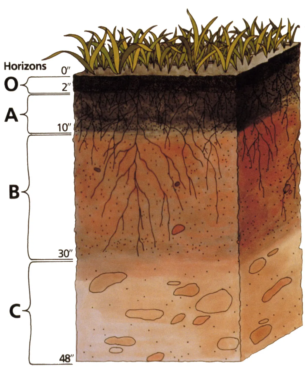
Curtis F. Marbut played a major role in adapting these ideas. In 1927 he published an English translation of Konstantin Glinka’s work, previously available in German. Attention increasingly centred on the sequence of horizons, their colour, structure and relationships. Chemistry and geology were incorporated into an account of soil formation, rather than discarded. The new perspective had limitations of its own: an excessive focus on an individual profile could obscure spatial variation. Further development required linking vertical sections with recurring arrangements of soils across slopes, terraces and plains.2
Classification and maps answer different questions
Marbut’s classifications and the system published in 1938 organised great diversity, but often relied on qualitative descriptions and interpretations of origin. Boundaries between classes could be uncertain. When classification required an explanation of how a soil formed, disagreements about its history could produce different assignments. Work on a new system under Guy Smith sought observable criteria and defined limits. It became the official system in 1965 and was published as Soil Taxonomy in 1975. Diagnostic horizons and properties made classification less directly dependent on a disputed reconstruction of genesis.
A taxonomic class defines a set of properties, whereas a map unit describes an actual part of the landscape. The two concepts are not interchangeable. Surveyors observe profiles at selected locations and use relationships between soils and landforms to infer conditions between them. Natural transitions may be gradual even though a map represents them at a particular scale. Nor does a class name itself specify crop yield or the current nutrient supply. Distinguishing taxonomy, mapping and interpretations for particular uses allowed the same evidence to serve several purposes without treating every description as an answer to the same question.23
Conservation and new ways to observe landscapes
During the twentieth century, farmers choosing crops ceased to be the only intended users. Surveys increasingly supported forestry, road construction, development and other decisions about land. Soil-conservation programmes of the 1930s increased demand for information about erosion, slope and limitations on use. Assessment required the kind of soil to be connected with its position and management. Mapping could provide a common evidential foundation, while the interpretation needed for a particular decision depended on the user’s purpose. The geographical record became relevant beyond the immediate question of agricultural production.
From the late 1930s and through the 1940s, aerial photographs became increasingly important base materials. Stereoscopic pairs assisted the recognition of relief, while visible fields, roads and streams helped locate observations. Photography supplied spatial context for points checked on the ground; it did not replace examination of profiles. Later orthophotographs reduced image distortions and improved connections to coordinate systems. Geographic information systems subsequently changed how observations were stored and compared. These tools expanded the handling of spatial evidence while preserving the need to understand soil-forming processes and verify interpretations in the field.2
Historical maps in a digital information system
For much of the programme’s history, the principal product was a printed report for a county or another survey area. It combined maps, descriptions and interpretations of suitability. Web Soil Survey became the official source of programme information in 2005, and the publication model based on printed editions progressively gave way to maintained digital datasets. Digitisation allowed surveys to be combined, boundaries revised and maps linked to descriptive databases. The change concerned the life cycle of information as well as the replacement of a paper sheet by a screen.
Historical reports remain evidence for the history of landscapes and agricultural knowledge. They record former soil names, crops, drainage practices and problems considered important by contemporary investigators. Reading them requires attention to the fieldwork date, scale and classification. Relatively persistent attributes coexist with properties altered by management, including organic carbon and structure. A comparison between an archival map and a later description can reveal environmental change, but also changes in methods and categories. Interpreting these records requires attention both to what earlier investigators observed and to the methods through which they understood the land.726
Questions and answers
Were the world’s first soil maps made in 1899?
No. Here 1899 refers to the opening field season of the US federal Soil Survey programme. Soil investigations and maps already existed in several countries, alongside earlier local work in the United States.25
Does a map colour show a field’s current fertility?
The colour identifies a unit defined by that map’s legend. It represents a recognised soil pattern rather than automatically specifying current nutrient levels or expected yield. Interpretation depends on scale, date and purpose.32
Why does the report for 1899 carry the date 1900?
Its title identifies the field season, while the publication date records the printing of the collected report. Individual maps could face additional delays: the report records the wait for a suitable base map for Cecil County.1
Sources
- Milton Whitney and collaborators, USDA Division of Soils (1900). Field Operations of the Division of Soils, 1899 — Report No. 64, printed by the Government Printing Office in 1900
- USDA Soil Science Division Staff (2017). Soil Survey Manual, Agriculture Handbook 18 — chapter 1, development of soil concepts, classification and survey
- USDA Soil Science Division Staff; chapter revised by Kenneth Scheffe and Shawn McVey (2017). Soil Survey Manual, Agriculture Handbook 18 — chapter 4, Soil Mapping Concepts
- David Rice Gardner (1957/1998). The National Cooperative Soil Survey of the United States — 1957 Harvard thesis, reprinted by USDA NRCS in 1998
- USDA Natural Resources Conservation Service (2024). Celebrate Soil Survey — 125th anniversary historical overview
- Terry J. Cosby, USDA Natural Resources Conservation Service (2024). Exploration, Invention and Evolution Still Abound after 125 Years of Soil Surveys
- USDA Natural Resources Conservation Service (n.d.). Soil Surveys by State — official description of historical printed surveys and the 2005 digital transition
Approximate dates (c.) describe the nature of the evidence: archaeology dates settlements, layers and remains, not single moments of invention.